Transport_program
Before starting, if you do not have it already, you will need to install the Graphite software (and its WarpDrive plugin, that is included in the distribution):
- if you are under Windows, install pre-compiled package (instructions here). The
WarpDriveplugin is included. - if you are under Linux or MacOS, install Graphite from sources (instructions here). You will need to compile the
WarpDriveplugin.
In this tutorial, we will use the LUA programming language. LUA is a scripting language similar to Python, if you know Python already you will (nearly) find yourself at home. More information about LUA here.
Why LUA rather than Python ?
-
LUA is smaller/faster/more elegantly designed (in my own subjective opinion). A more objective measure: it has a super small footprint (in terms of source size, package size). It is directly included in Graphite (nothing to install).
-
If you really prefer Python (that is much more popular than LUA and that has many existing packages), there will be a Python version of this tutorial soon (Graphite also supports Python through the "gompy" plugin).
Now you can take a quick look at the Scripting Graphite tutorial to see how the editor works (see in particular automatic completion and help bubbles that can save you some time).
We shall now see how to create a Laguerre diagram in Graphite and how to visualize it.
The first thing we need to do is defining the
domain. We create a unit square, using the create_square() method of
the Shapes interface. Then we need to triangulate the domain (this
will simply split the square into two triangles in our case).
scene_graph.clear()
Omega = scene_graph.create_object('OGF::MeshGrob')
Omega.rename('Omega')
Omega.I.Shapes.create_square()
Omega.I.Surface.triangulate()
Omega.visible = falseNow we create a point set. In this example, we will use a set
of N=100 points picked randomly in our unit square:
N = 100 -- Number of points
Omega.I.Points.sample_surface(
   {nb_points=N,Lloyd_iter=0,Newton_iter=0}
)
points = scene_graph.objects.pointsAnd finally, we can compute the Laguerre diagram (restricted
to the domain). We first create a new mesh to store it.
Laguerre diagrams are defined from a pointset and a vector
of "weights". Here we use (for now) a vector of weights with
all weights set to 0 (default value set by NL.create_vector()).
RVD = scene_graph.create_object('OGF::MeshGrob','RVD')
weight   = NL.create_vector(N)
Then we can compute the Laguerre diagram. The WarpDrive plugin
adds a special Transport interface solely designed for scripting
(it does not appear in the menus). It has a function to compute
the Laguerre diagram:
points.I.Transport.compute_Laguerre_diagram(
   Omega, weight, RVD, 'EULER_2D'
)And finally, we can set the graphic attributes of the computed Laguerre diagram to display the cells in different colors:
RVD.shader.painting='ATTRIBUTE'
RVD.shader.attribute='facets.chart'
RVD.shader.colormap = 'plasma;false;732;false;false;;'
RVD.shader.autorange()
The complete program is available here. You can also load it from the Examples... menu of the text editor (Examples.../WarpDrive/advanced/Transport_2d_01.lua).

Let us now see what happens when we change the weight of one cell in the Laguerre diagram. For that, we
write a function compute(), at the beginning of our file as follows:
function compute()
   weight[0] = weight[0] + 0.01
   OT.compute_Laguerre_diagram(Omega, weight, RVD, 'EULER_2D')
   RVD.shader.autorange()
   RVD.update()
end
Now we want to create a button that will call our function compute() each time we push it.
At the end of our file, we add:
OT_dialog = {}
OT_dialog.visible = true
OT_dialog.name = 'Transport'
OT_dialog.x = 100
OT_dialog.y = 400
OT_dialog.w = 150
OT_dialog.h = 200
OT_dialog.width = 400

function OT_dialog.draw_window()
   if imgui.Button('Compute',-1,-1) then
      compute()
   end
end

graphite_main_window.add_module(OT_dialog)
This declares a new Module to the graphic user interface of Graphite. See
the Scripting Graphite tutorial for more details. Each time the
Compute button is pressed, our function compute() is called. It increases
a bit the weight of one of the points and recomputes the Laguerre diagram, so
that you can see the impact of modifying the weight of a single point.
The complete program is available here. You can also load it from the Examples... menu of the text editor (Examples.../WarpDrive/advanced/Transport_2d_02.lua).
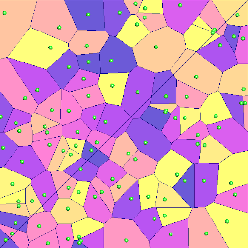
Run the program (<F5>), then push the compute button multiple times, you will see one of the cells growing bigger and bigger. It will eventually
nibble the entire domain (all the other cells become eventually empty, yes a Laguerre diagram can have empty cells).
![]()
Now you may think about a Laguerre diagram as a Voronoi diagram plus tuning buttons (the weights). By changing the tuning buttons, one may increase or decrease the size of the associated Laguerre cells. In fact there is more: did you know that you can translate a Laguerre diagram by an arbitrary vector just by changing the weights ?
Let us take a close look at the common boundary between two cells i and j,
associated with points xi and xj.
A point x that is on this common boundary satisfies the following equation:
where wi and wj are the weights associated with points xi and xj and
where d2(.,.) denotes the squared distance between two points.
Side note: One can notice that this equation only involves linear terms in the coordinates of x (the
squared lengh of x appears on both sides of the equation and cancel out), hence this
common boundary is a straight line.
Suppose that wi = wj = 0, then what you have is the Voronoi diagram of xi and xj.
Imagine now that you want to translate the whole diagram by an arbitrary 2D vector T. Is
is possible to do so just by changing wi and wj ?
Try to derive it on your own before reading further
In other words, how can we set wi and wj in such a way that the set of
points x that satisfy:
corresponds to the same straight line as the edge between the Voroonoi cells of xi and xj ?
It can be easily checked that setting wi = -2(T.xi) and wj = -2(T.xj) works (where . denotes
the dot product).
OK, let us now program it !
First thing we need to do is to group a little bit our points in the lower-left corner of the square,
so that we will still see them when we will translate them. Right after we create the point set, we
declare a mesh editor (E = points.I.Editor), find the attribute that stores the point coordinates
(coords = E.find_attribute('vertices.point')) and modify the coordinates:
  E = points.I.Editor
  coords = E.find_attribute('vertices.point')
  for i=0,N-1 do
     coords[3*i]   = coords[3*i]/2.0
     coords[3*i+1] = coords[3*i+1]/2.0
  end
Then, we will keep the same graphic interface (the big Compute button), and change the compute() function
as follows:
  Tx = 0.0
  Ty = 0.0
  function compute()
     Tx = Tx + 0.05
     Ty = Ty + 0.05
     for i=0,N-1 do
        weight[i] = - 2.0 * Tx * coords[3*i]
                    - 2.0 * Ty * coords[3*i+1]
     end
     OT.compute_Laguerre_diagram(Omega, weight, RVD, 'EULER_2D')
     RVD.shader.autorange()
     RVD.update()
   end
The complete program is available here. You can also load it from the Examples... menu of the text editor (Examples.../WarpDrive/advanced/Transport_2d_03.lua).
Run the program (<F5>), then push the compute button multiple times, you will see the whole diagram moving towards the upper-right corner.
What we have learnt so far:
- how to compute a Laguerre diagram in Graphite
- by changing the weights of a Laguerre diagram, one can change the area of the cells
- by changing the weights of a Laguerre diagram, one can translate it at a arbitrary position

Semi-discrete Optimal Transport gives a way of computing the weights in such a way that all the cells
have prescribed areas. As before, we will start from a random distribution of points, and from their
Voronoi diagram (all weights set to zero). Then we will iteratively update the weights until all
the Laguerre cells have the prescribed areas (it will be the same, nu_i=1/N', for all cell iin the present example). For now, we want to do one updating step each time theCompute` button is pressed.
We just need to change the compute() function of our previous program, to make it compute one Newton
step. We know (detailed derivation here) that this means solving
a discrete Poisson system. Warpdrive has a function to assemble the Poisson system for you (we will see
lated how to do that on our own), as follows:
  function compute()
     local L = NL.create_matrix(N,N) -- P1 Laplacian of Laguerre cells
     local b = NL.create_vector(N)   -- right-hand side
     OT.compute_Laguerre_cells_P1_Laplacian(
        Omega, weight, L, b, 'EULER_2D'
     )
     ...
  end
This creates a sparse matrix L with the discrete Laplacian corresponding to the current
Laguerre diagram, and initializes the vector b with the areas of the Laguerre cells.
See also the scripting tutorial
about linear algebra in Lua.
Then we need to initialize the right-hand side b of our Poisson system. Each component of b
is supposed to be equal to the target area (nu_i=1/N in our case) minus the current area of the
Laguerre cell. Hence we update b as follows (still in the same compute() function):
   ...
   for i=0,N-1 do
     local nu_i = 1.0/N  -- desired area for Laguerre cell i
     b[i] = nu_i - b[i]  -- rhs = desired area - actual area
   end
   ...
Then we solve the linear system:
   ...
   local p = NL.create_vector(N)   -- Newton step vector
   L.solve_symmetric(b,p)          -- solve for p in Lp=b
   ...
This gives us a Newton step vector p. We still do not know
how much along p we should descend, for now we descend by
a fixed parameter alpha=1/8 (more on this later):
   ...
   local alpha = 1.0/8.0           -- Steplength (constant for now)
   NL.blas.axpy(alpha, p, weight)  -- weight = weight + alpha * p
   ...
Putting everything together, our new compute() function looks like that:
function compute()
   -- compute L(Laplacian) and b(init. with Laguerre cells areas)
   local L = NL.create_matrix(N,N) -- P1 Laplacian of Laguerre cells
   local b = NL.create_vector(N)   -- right-hand side
   OT.compute_Laguerre_cells_P1_Laplacian(
      Omega, weight, L, b, 'EULER_2D'
   )

   for i=0,N-1 do
     local nu_i = 1.0/N  -- desired area for Laguerre cell i
     b[i] = nu_i - b[i]  -- rhs = desired area - actual area
   end

   local p = NL.create_vector(N)   -- Newton step vector
   L.solve_symmetric(b,p)          -- solve for p in Lp=b
   local alpha = 1.0/8.0           -- Steplength (constant for now)
   NL.blas.axpy(alpha, p, weight)  -- weight = weight + alpha * p

   OT.compute_Laguerre_diagram(Omega, weight, RVD, 'EULER_2D')
   RVD.shader.autorange()
   RVD.update()
end
The complete program is available here. You can also load it from the Examples... menu of the text editor (Examples.../WarpDrive/advanced/Transport_2d_04.lua).
- Run the program (
<F5>), then push thecomputebutton multiple times, you will see that it converges to a Laguerre diagram with the same area for all the cells. - Set
shrink_pointstotrue, run the program then push thecomputebutton multiple times. This will show a more extreme change of cells area. As you can see, in a Laguerre diagram, a point does not necessarily belong to its cell (unlike Voronoi diagrams).
Now try this: set shrink_points to true, and divide point coordinates by 10 (instead of 2):
...
   if shrink_points then
      for i=0,N-1 do
         coords[3*i]   = 0.25 + coords[3*i]/10.0
         coords[3*i+1] = 0.25 + coords[3*i+1]/10.0
      end
   end
...
Now run the program, and push the Compute button a couple of time. As you can see, it no longer converges. Can you find a quick-and-dirty fix for this
example ?
OK, let us try with a smaller alpha, let us say alpha=1.0/10.0 ? No, does not converge, and what about alpha=1.0/100.0 ? Yes, it does the right thing.
Now, it would not be reasonable to let the user tune alpha, so let us move to the next step !

There is a nice article by Jun Kitagawa, Quentin Merigot and Boris Thibert, with a method
(called "KMT" after its authors) to choose alpha in such a way that the convergence of the Newton method is guaranteed.
The idea is to start with alpha=1, then halve alpha until certain conditions are satisfied. These conditions says that:
- all Laguerre cells should be larger than half the smallest Voronoi cell
- all Laguerre cells should be larger than half the smallest target area (
0.5/Nin our case) - the norm of
gafter the update should be smaller than(1 - 0.5*alpha)*norm(g)before the update, wheregis the vector of the differences between the target areas and the actual areas of the Laguerre cells (g_i = nu_i - Area(Lag(i)) = 1/N - Area(Lag(i)))
Remark the first condition forbids to have any empty Laguerre cell in the diagram.
Now we can update our compute() function to take into account the three KMT conditions. For the first two ones,
we need to compute the area of the smallest Voronoi cell. Since the first iteration computes a Voronoi diagram
(all weights set to zero), we compute it right after:
smallest_cell_threshold = -1.0

function compute()
   ...
   -- compute minimal legal area for Laguerre cells (KMT criterion #1 and #2)
   -- (computed at the first run, when Laguerre diagram = Voronoi diagram)
   if smallest_cell_threshold == -1.0 then
      local smallest_cell_area = b[0]
      for i=1,N-1 do
         smallest_cell_area = math.min(smallest_cell_area, b[i])
      end
      smallest_cell_threshold =
         0.5 * math.min(smallest_cell_area, 1.0/N)
      print('smallest cell threshold = '..tostring(smallest_cell_threshold))
   end
   ...
Then we solve the Newton step vector p as before, and
we compute several trial weight vectors weight2 and test the three KMT conditions:
   local alpha = 1.0
   local weight2 = NL.create_vector(N)
   local g_norm = NL.blas.nrm2(b)  -- squarred norm of gradient at current step

   -- Divide steplength by 2 until both KMT criteria are satisfied
   for k=1,10 do
      NL.blas.copy(weight, weight2)
      NL.blas.axpy(alpha, p, weight2) -- weight2 = weight + alpha * p
      OT.compute_Laguerre_cells_measures(Omega, weight2, b, 'EULER_2D')
      local smallest_cell_area = b[0]
      for i=1,N-1 do
         smallest_cell_area = math.min(smallest_cell_area, b[i])
      end

      -- Compute squarred gradient norm at current substep
      local g_norm_substep = 0.0
      for i=0,N-1 do
         local g_i = b[i] - Omega_measure/N
         g_norm_substep = g_norm_substep + g_i * g_i
      end
      g_norm_substep = math.sqrt(g_norm_substep)

      if (smallest_cell_area > smallest_cell_threshold) and
         (g_norm_substep <= (1.0 - 0.5*alpha) * g_norm) then
         break
      end

      alpha = alpha / 2.0
   end

   NL.blas.copy(weight2, weight)
The complete program is available here. You can also load it from the Examples... menu of the text editor (Examples.../WarpDrive/advanced/Transport_2d_05.lua).
- Run the program (
<F5>), then push thecomputebutton multiple times. You will see in the console how many substeps are used. - Try setting
Nto 10000, and re-run the program. - Try dividing the coordinates more (by 100) and re-run the program. No longer converges, can you guess why ? Can you fix it ?
(hint: it may need more than 10 substeps to find the right value of
alpha).
The MKT algorithm is very robust and still works for configurations with all the points nearly at the same position !

Up to know, we have supposed a uniform density in the domain. Let us see how to compute optimal transport with a domain that has a spatially varying density. It means that instead of the area of the cells, what we constrain is the integrated density over each cell.
We first create the domain. Before calling triangulate, with split the
domain into a 32x32 grid:
   Omega = scene_graph.create_object('OGF::MeshGrob','Omega')
   Omega.I.Shapes.create_square()
   Omega.I.Surface.split_quads(5)
   Omega.I.Surface.triangulate()
Then we create the attribute, initialize it using a formula and display it:
   E = Omega.I.Editor
   coords = E.find_attribute('vertices.point')
   density = E.create_attribute('vertices.weight')
   for i=0,#density-1 do
      local x = coords[3*i]
      local y = coords[3*i+1]
      local s = 0.5 * (1.0 + math.sin(x*10) * math.sin(y*10))
      density[i] = 0.001 + s*s
   end
   Omega.shader.painting='ATTRIBUTE'
   Omega.shader.attribute='vertices.weight'
   Omega.shader.colormap = 'plasma;false;1;false;false;;'
   Omega.shader.autorange()
The presence of the density attribute (attached to the vertices of the domain, and
called weight - not to be confused with the weights of the Laguerre diagram - is
detected by all the functions of the OptimalTransport interface.
The only thing that needs to be changed is that now the total area of the domain (1) needs
to be replaced with the integrated density attribute over the domain:
   Omega_measure = OT.Omega_measure(Omega, 'EULER_2D')
   ...
   nu_i = Omega_measure / N
The complete program is available here. You can also load it from the Examples... menu of the text editor (Examples.../WarpDrive/advanced/Transport_2d_06.lua).

- Run the program (
<F5>), then push theComputebutton. You will see the diagram evolve to match the density attribute. - Run the program again (
<F5>), then hideOmegain the object list, then push theComputebutton again to better see the Laguerre cells. - Set
shrink_pointstotrue, run the program again, push theComputebutton again.
The last run (shown in the video above) is a quite challenging configuration. KMT step-length control does a good job, and finally converges to the correct solution.
Up to now, we have been using the OT.compute_Laguerre_cells_P1_Laplacian() function to assemble the sparse matrix of the linear system and
compute the area of the Laguerre cells. Let us see how it works under the hood, and implement our own version in LUA !
We first need a couple of helper functions, that compute the distance between two vertices in a mesh, and the area of a triangle in a mesh:
function distance(XYZ, v1, v2)
  local x1 = XYZ[3*v1]
  local y1 = XYZ[3*v1+1]
  local x2 = XYZ[3*v2]
  local y2 = XYZ[3*v2+1]
  return math.sqrt(
    (x2-x1)*(x2-x1) + (y2-y1)*(y2-y1)
  )
end

function triangle_area(XYZ, v1, v2, v3)
  local x1 = XYZ[3*v1]
  local y1 = XYZ[3*v1+1]
  local x2 = XYZ[3*v2]
  local y2 = XYZ[3*v2+1]
  local x3 = XYZ[3*v3]
  local y3 = XYZ[3*v3+1]
  return math.abs(
    0.5 *(
      (x2-x1)*(y3-y1) - (y2-y1)*(x3-x1)
    )
  )
end
The first argument XYZ is the vector of all vertices coordinates.
Now, still following the derivation here, we can assemble our Poisson system as follows:
-- Computes the linear system to be solved at each Newton step
-- This is a LUA implementation equivalent to the builtin (C++)
--   OT.compute_Laguerre_cells_P1_Laplacian(
--      Omega, weight, H, b, 'EULER_2D'
--   )
-- H the matrix of the linear system
-- b the right-hand side of the linear system
function compute_linear_system(H,b)

   -- Get the Laguerre diagram (RVD) as a triangulation
   OT.compute_Laguerre_diagram(Omega, weight, RVD, 'EULER_2D')
   RVD.I.Surface.triangulate()
   RVD.I.Surface.merge_vertices()

   -- vertex v's coordinates are XYZ[3*v], XYZ[3*v+1], XYZ[3*v+2]
   XYZ   = RVD.I.Editor.find_attribute('vertices.point')

   -- Triangle t's vertices indices are T[3*t], T[3*t+1], T[3*t+2]
   T     = RVD.I.Editor.get_triangles()

   -- The indices of the triangles adjacent to triangle t are
   --    Tadj[3*t], Tadj[3*t+1], Tadj[3*t+2]
   --  WARNING: they do not follow the usual convention for triangulations
   --  (this is because GEOGRAM also supports arbitrary polygons)
   --
   -- It is like that:
   --
   --        2
   --       / \
   -- adj2 /   \ adj1
   --     /     \
   --    /       \
   --   0 ------- 1
   --      adj0
   --
   -- (Yes, I know, this is stupid and you hate me !!)

   Tadj  = RVD.I.Editor.get_triangle_adjacents()

   -- chart[t] indicates the index of the seed that corresponds to the
   --  Laguerre cell that t belongs to
   chart = RVD.I.Editor.find_attribute('facets.chart')

   -- The coordinates of the seeds
   seeds_XYZ = points.I.Editor.find_attribute('vertices.point')

   -- The number of triangles in the triangulation of the Laguerre diagram
   local nt = #T/3

   -- For each triangle of the triangulation of the Laguerre diagram
   for t=0,nt-1 do

     -- Triangle t is in the Laguerre cell of i
     local i  = chart[t]

     -- Accumulate right-hand side (Laguerre cell areas)
     b[i] = b[i] + triangle_area(XYZ,T[3*t], T[3*t+1], T[3*t+2])

     --   For each triangle edge, determine whether the triangle edge
     -- is on a Laguerre cell boundary and accumulate its contribution
     -- to the Hessian

     for e=0,2 do
         -- index of adjacent triangle accross edge e
         local tneigh = Tadj[3*t+e]

	 -- test if we are not on Omega boundary
	 if tneigh < nt then

	    -- Triangle tneigh is in the Laguerre cell of j
	    local j = chart[tneigh]

	    -- We are on a Laguerre cell boundary only if t and tneigh
	    -- belong to two different Laguerre cells
	    if not (j == i) then

	       -- The two vertices of the edge e in triangle t
	       local v1 = T[3*t+e]
	       local v2 = T[3*t+((e+1)%3)]

	       local hij = distance(XYZ,v1,v2) / (2.0 * distance(seeds_XYZ, i,j))
	       H.add_coefficient(i,j,-hij)
	       H.add_coefficient(i,i,hij)
	    end
	 end
     end
   end
end
The function OT.compute_Laguerre_diagram() creates the Laguerre diagram, and decomposes all the
cells into triangles. Then we use a MeshEditor to access several arrays:
- the vertices coordinates
XYZ - the triangles array
T - the triangles adjacency array
T_adj - the index of the cell each triangle belongs to
chart - the coordinates of the initial points from which we computed the Laguerre diagram
seeds_XYZ
From this information, it computes the areas of the cells in the b vector, and the coefficients of
the Laplacian in the H sparse matrix, defined by:
h_ij = -length(B_ij) / 2 * distance(x_i, x_j)-
h_ii = -sum_j(h_ij)where B denotes the edge common to cellsiandj.
The complete program is available here. You can also load it from the Examples... menu of the text editor (Examples.../WarpDrive/advanced/Transport_2d_07.lua).